


What Permit-to-Spud Ratios Reveal About County Activity
Natural gas developers do not drill every tract they permit. A dense stack of drilling notices can mean either a large future drilling campaign or paperwork that never reaches the rig. The ratio of permits to spuds reveals how much of that apparent momentum is becoming actual well activity. It is most useful as a trend and diagnostic, not as a stand-alone score.
For Australian teams working from Sydney or Melbourne, county data can benchmark US unconventional gas exposure before an investment committee reviews acreage, gathering costs or counterparty risk. The measure needs careful construction, however: permits and spuds must cover matching periods, map to the same geography and use consistent permit definitions. Read that way, it can expose directional shifts in operator appetite, pipeline depth and local execution.
Why the ratio matters
The simplest version divides permits approved during a period by wells spudded, meaning drilling begun, during that same period. A result of 2.0 means two permits for every spud; 0.5 means one permit for every two spuds. Because both sides are flows rather than a complete inventory, the result describes current throughput, not the number of ready-to-drill locations.
A ratio above 1 can indicate that operators are acquiring drilling positions faster than they convert them into wells. That may foreshadow a busier rig schedule, provided permits remain valid and crews are available. A ratio below 1 can indicate a spudding catch-up, older approvals entering the field, or a pause in new permit activity. The same number can therefore carry different meanings across counties.
Build a comparable county measure
Start with dates and cohort logic. For a flow view, count approvals and spuds over the same 90-day, quarterly or annual window. For a cohort view, follow permits approved during one period and record whether and when they became spuds. Comparing new permits this quarter with wells drilled last quarter can manufacture a false surge when rigs arrive late after a permit cohort was assembled.
Confirm what each record represents. Some permit datasets include pending applications while others show issued approvals; lease offers form a separate layer, and a transfer or renewal may create another row without another drilling location. The spud side should be checked against Shale Navigator's well records, using operator, date, well type and location details to remove duplicate or out-of-area entries. Also determine whether one approval can cover multiple wells or a multi-well pad.
Geography must also be stable. A county boundary change, annexed township or well located near a lease-line can shift counts without any change in drilling. Use one authoritative boundary for both datasets and decide explicitly whether the unit is the permit location, the wellhead or the operating company before calculating the ratio.
Interpret high and low readings
A sustained increase in permits alongside rising spuds suggests active expansion. The important question is the lag: if spuds trail approvals by two quarters, the operator may be building a workload; if both move together, crews may be converting positions promptly. A widening gap deserves attention when rig availability, equipment queues or pressured decline is tight.
A falling spud count with steady permit issuance can point to execution constraints rather than weak land demand. Check whether operators are prioritising better acreage, waiting for a shared pad, or preserving cash after a commodity-price move. By contrast, a low ratio caused by a temporary permit surge is not inherently bearish if the relevant operator has a credible near-term spud schedule.
Do not infer growth from one volatile county. Combine the ratio with absolute counts, acreage concentration and multi-period trends. Ten permits and five spuds is a ratio of 2.0, yet the absolute workload may be modest; a larger county can show 1.2 with far greater drilling volume. Ratios clarify relationships, while counts retain scale.
Connect the measure to operator behaviour
Operator mix changes the interpretation. Several small companies filing permits may fragment the workload and compete for the same limited rig and frac crews. A dominant operator with an established local footprint may convert permits more consistently but also dominate the county risk profile. Compare permit-to-spud conversion by operator, where coverage permits, and preserve the identity of permit holders rather than relying only on acreage totals.
The pattern also speaks to capital discipline. Repeated permits with few spuds may reflect a land-buying phase, option strategies or approvals held for a later window. Strong conversion can reveal operational momentum, yet it does not guarantee economic success. Evaluate drilling depth, completion design, pipeline takeaway, water availability and expected well productivity alongside the permit ratio, because a fast spudding pace can still create uneconomic wells.
Account for local and Australian context
US counties differ in road access, pipeline reach, water constraints, weather windows and proximity to service basins. A county with fewer permits may have stronger gathering infrastructure, while a heavily permitted frontier county may face long equipment hauls. Interpret the signal against those operating conditions and against the operator's broader portfolio, since company-level strategy can outweigh local geology in any single quarter.
Australian readers should not translate a US county directly into state acreage. Mineral rights, land access, royalty arrangements and approvals in Queensland, New South Wales and Western Australia operate under different frameworks from US county records. Native-title consultation and environmental conditions can also materially affect timing, making a permit count in those markets less comparable without tenure and approval data.
For teams based in Sydney or Melbourne, the practical value of US county analysis is a screening tool for cross-border holdings. It can sit alongside ASX company announcements, AUD-denominated capital commitments and USD oilfield service contracts. Australian energy investors should also preserve currency and fiscal context when comparing US basins, since federal, state and local rules do not mirror Australia's royalty and tenement systems.
Apply a county activity checklist
A useful review should separate the signal from its causes. Record the calculation window, permit definition and geography first, then investigate what changed in the operator roster, rig market or local infrastructure.
Signals to examine
- Permits rising while spuds remain flat indicates a possible future drilling queue.
- Permits and spuds rising together points to active expansion, subject to normal timing lags.
- Spuds falling while permits hold steady may signal scheduling, service or capital constraints.
- More permit holders than spudding operators can indicate workload fragmentation and rig-access pressure.
Records to verify
- Match approval and spud dates to the same reporting window.
- Exclude pending, cancelled, transferred or duplicated permit records.
- Separate vertical, horizontal and appraisal wells where relevant.
- Apply one county boundary to both permit locations and wellheads.
Finish by separating a county-wide signal from operator-specific evidence. Review the companies holding the permits, their rig commitments and the acreage behind each approval. A ratio that looks weak across the county may be strong for one operator, while an apparently strong county ratio may conceal a narrow group carrying all activity.
Turn the signal into a decision
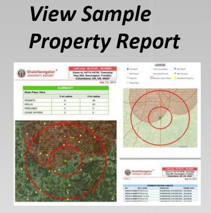
Shale Navigator's platform overview describes the map layers available for analysing permits, pipelines, lease offers, mineral rights and property context. Combine those layers with the permit-to-spud measure, then compare several quarters rather than reacting to a single week's movement. This creates a clearer chain from land acquisition to drilling intent and field execution.
Open a seven-day account, identify the counties and operators driving the change, and test the pattern against rig access, acreage quality and infrastructure constraints. Use the result to prioritise deeper diligence, direct land and well-data reviews, or schedule operator conversations where the conversion gap is most significant.