Tracking Monthly Rig Movement Across Major Shale Plays

Mapping the monthly change in active rigs across major U.S. shale plays turns a headline number into a geographic view of where crews, equipment and drilling capital are moving. An active rig is normally recorded as working at a defined time, but datasets may count drilling, completion or both. The source definition should travel with every map rather than sit in a footnote.

Monthly movement is an operational signal rather than a direct measure of gas or oil output. A new rig can indicate development, while a removed rig may reflect a completed well, equipment relocation or a temporary pause. Consistent month-over-month comparisons reveal shifts in operator attention and help users identify where permits, mineral positions, infrastructure and local research deserve closer attention.

What an Active Rig Actually Measures

An active rig generally means a unit with a crew and equipment in operation at the reporting cut-off. Some services publish a month-end count, while others calculate a monthly average from weekly observations. Those methods produce different results around month boundaries, so every report should state the observation rule, time zone and treatment of stacked or completion rigs.

A count also says little about well quality, lateral length or reservoir stage. In mixed oil-and-gas plays, a growing oil-directed fleet can coincide with flat or declining gas activity. Use rig movement to locate change, then test it against production, completions and well-cost evidence before treating it as a forecast.

Establishing the Monthly Comparison

Begin with a fixed play definition. The Permian can be divided into the Delaware and Midland platforms, Anadarko into its principal shale counties, and the Haynesville into its Texas-Louisiana footprint. Keep those choices unchanged between reporting periods; otherwise, a boundary revision can resemble genuine month-over-month growth. Counties can overlap several plays, so each rig should be allocated once to the selected play and multi-play locations should be flagged separately.

Choose one cut-off for every basin and preserve the original timestamp. Australian teams must account for Brisbane’s year-round Eastern Standard Time, Sydney’s daylight-saving changes and Perth’s Western Standard Time, then compare them with the Central Time convention commonly used by U.S. rig services. A Perth analyst checking reports before the office opens is reviewing activity under a different clock from a Brisbane-based gas desk.

Record net change, percentage change and the starting count. Net change equals the current count minus the previous count; percentage change divides that difference by the earlier count. A move from 40 rigs to 36 is a loss of four, or 10 per cent, while a move from 40 to 44 is a gain of four, or 10 per cent. Starting totals matter because the same numerical movement carries different weight in a small gas play and a large oil basin.

Turning Counts Into Spatial Change

Map each monthly total at play level first, then examine the counties or operating districts where movement occurred. Graduated symbols can represent the current count, the percentage change or both, while a neighbouring table provides exact figures. Keep the scale consistent through time. For basin-scale interpretation, normalising the rig count by active well inventory or developed acreage can show whether activity is becoming more concentrated rather than simply holding steady.

A useful monthly briefing distinguishes additions, removals and areas with little movement. Growth on the edge of a core county may indicate newer acreage, while growth near existing infrastructure can suggest an infill programme. These remain interpretations rather than certainties: a rig can relocate to a multi-well pad, and permit activity may precede drilling by months.

Adding the Shale Navigator Layers

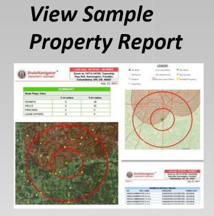
A rig point becomes more useful when viewed with the play outline, producing counties, pipelines and available mineral rights. Shale Navigator places these layers alongside drilling permits and property information, allowing analysts to consider whether activity has road access, takeaway capacity and a plausible land position. Spatial overlap creates a question for further investigation rather than proof that every supporting interest is secure.

Historic wells can complicate a proposed lateral even when the active-rig total is rising. A historic vertical well review can help identify old vertical wells, plugging records and spacing constraints that may affect a horizontal path. Engineers and landmen can then check the findings against current surveys and operator files instead of relying on a production map alone.

Each layer also needs a clear status label. A permit represents authorisation, an advertised lease offer remains a proposed transaction until confirmed, and a pipeline line may be planned or operational. None automatically proves present drilling, completed title or available transport capacity. This distinction protects mineral-rights investors from treating proximity on a map as a completed legal or commercial arrangement.

Reading the Direction of Movement

Increases often suggest that operators expect sufficient acreage, service capacity or commodity prices to keep rigs working, but the underlying cause can differ by company. Compare additions with lease sales, permit cadence, reservoir pressures and infrastructure arrivals. A broad rise becomes more persuasive when it persists across several reporting periods and coincides with stable well productivity rather than falling performance.

Falls can also provide useful evidence. They may indicate maturing core acreage, weaker commodity expectations, infrastructure delays or relocation of equipment to a more attractive basin. Read declines alongside inventories and permitting before labelling them as field exhaustion. For Australian energy users, a Brisbane team working across domestic gas or Queensland LNG can add market context, while recognising that Australia has no commercial shale gas play at U.S. scale and that the two industries have different geology, contracts and fiscal settings.

Making the Map Work Across Disciplines

Different users require different follow-up. Engineers can compare rig locations with spacing and infrastructure, landmen can review ownership and access, investors can assess operator and royalty exposure, and government or university teams can study regional concentration. A shared map should retain its source, date and methodology so each group can reproduce the analysis without quietly changing definitions or boundaries.

Australian conventions deserve explicit labels. Many local reports use hectares, while U.S. mineral records commonly use acres, making a 40-acre interest approximately 16.2 hectares. Coordinate systems also differ: Australian mapping commonly uses GDA94, whereas U.S. layers generally use NAD83 or another state-defined system. Australian native-title and land-access questions may engage the Native Title Act 1993 and state legislation. Those laws do not determine title to a U.S. parcel, but they reinforce the need to separate analytical map evidence from legal due diligence.

If the available layer or licence coverage is unclear, send the project question through the Navigator contact page before the team sets monitoring thresholds.

Create a free seven-day Shale Navigator account, select one well-defined play and build its first two-month comparison before expanding the review. Standardise the cut-off, count method, boundaries and supporting layers, then archive the result as a repeatable baseline. Additional data and features are available through subscriptions as the monitoring programme develops. Open the account and build that first comparison now.